In this proof we (finally!) finish the proof of case one.
As usual, we throughout fix a nonstandard natural  and a complex polynomial of degree whose zeroes are all in
  . We assume that
  is a zero of
  whose standard part is
  , and assume that has no critical points in
  . Let
. Let  be a random zero of and
  a random critical point. Under these circumstances,
  is uniformly distributed on
  and
and  is almost surely zero. In particular,
and is infinitesimal in probability, hence infinitesimal in distribution. Let  be the expected value of (thus also of ) and
  its variance. I think we won’t need the nonstandard-exponential bound
  this time, as its purpose was fulfilled last time.
Last time we reduced the proof of case one to a sequence of lemmata. We now prove them.
1. Preliminary bounds
Lemma 1 Let  be a compact set. Then

uniformly for  .
.
Proof: It suffices to prove this for a compact exhaustion, and thus it suffices to assume

By underspill, it suffices to show that for every standard  we have

We first give the proof for  .
.
First suppose that  . Since is infinitesimal in distribution,

here we need the  and the
  since
since  is not a bounded continuous function of . Since
  we have

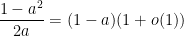
but we know that

so, solving for  , we get

we absorbed a  into the
  . That gives

Since is a polynomial of degee  and is monic (so the top coefficient of is ) this gives a bound
even for  .
.
Now for , we use the bound
to transfer the above argument. 
2. Uniform convergence of
Lemma 2 There is a standard compact set  and a standard countable set
  such that

all elements of  are isolated in
  , and
, and  is infinitesimal.
Tao claims

where  is a large standard natural, which makes no sense since the left-hand side should be large (and in particular, have positive standard part). I think this is just a typo though.
Proof: Since was assumed far from  we have

We also have

so for every standard natural there is a standard natural  such that

Multiplying both sides by we see that

where  is the variety of critical points
  . Let
. Let  be the set of standard parts of zeroes in
  ; then has cardinality
  and so is finite. For every zero
  , either
- For every ,

so the standard part of  is , or
- There is an such that
 is infinitesimal.
So we may set  ; then is standard and countable, and does not converge to a point in
  , so is standard and is infinitesimal.
I was a little stumped on why is compact; Tao doesn’t prove this. It turns out it’s obvious, I was just too clueless to see it. The construction of forces that for any , there are only finitely many  with
with  , so if clusters anywhere, then it can only cluster on . This gives the desired compactness.
The above proof is basically just the proof of Ascoli’s compactness theorem adopted to this setting and rephrased to replace the diagonal argument (or 👏 KEEP 👏 PASSING 👏 TO 👏 SUBSEQUENCES 👏) with the choice of a nonstandard natural. I think the point is that, once we have chosen a nontrivial ultrafilter on  , a nonstandard function is the same thing as sequence of functions, and the ultrafilter tells us which subsequences of reals to pass to.
3. Approximating  outside of
We break up the approximation lemma into multiple parts. Let  be a standard compact set which does not meet . Given a curve
  we denote its arc length by
  ; we always assume that an arc length does exist.
A point which stumped me for a humiliatingly long time is the following:
Lemma 3 Let  . Then there is a curve from
  to
to  which misses and satisfies the uniform estimate

Proof: We use the decomposition of into the arc
and the discrete set . We try to set to be the line segment ![{[z, w]}](https://s0.wp.com/latex.php?latex=%7B%5Bz%2C+w%5D%7D&bg=ffffff&fg=000000&s=0&c=20201002) but there are two things that could go wrong. If hits a point of we can just perturb it slightly by an error which is negligible compared to . Otherwise we might hit a point of
but there are two things that could go wrong. If hits a point of we can just perturb it slightly by an error which is negligible compared to . Otherwise we might hit a point of  in which case we need to go the long way around. However, and are compact, so we have a uniform bound
Therefore we can instead consider a curve which goes all the way around , leaving  . This curve has length
  for
for  close to (and if are far from we can just perturb a line segment without generating too much error). Using our uniform max bound above we see that this choice of is valid.
Recall that the moments  of are infinitesimal.
Since is infinitesimal, and is a positive distance from any infinitesimals (since it is standard compact), we have

uniformly in . Therefore has no critical points near and so  is holomorphic on .
We first need a version of the fundamental theorem.
Lemma 4 Let be a contour in of length . Then

Proof: Our bounds on  imply that we can take the Taylor expansion

of in terms of , which is uniform in . Taking expectations preserves the constant term (since it doesn’t depend on ), kills the linear term, and replaces the quadratic term with a , thus

At the start of this series we showed

Plugging in the Taylor expansion of  we get

Simplifying the integral we get

whence the claim.
Lemma 5 Uniformly for  one has

Proof: Applying the previous two lemmata we get

It remains to simplify

Taylor expanding  and using the self-similarity of the Taylor expansion we get

which gives that bound.
Lemma 6 Let . Then

uniformly in .
Proof: We may assume that  is small enough depending on , since the constant in the big-
 notation can depend on as well, and only appears next to implied constants. Now given we can find from to
  which is always moving at a speed which is uniformly bounded from below and always moving in a direction towards the origin. Indeed, we can take to be a line segment which has been perturbed to miss the discrete set , and possibly arced to miss (say if is far from ). By compactness of we can choose the bounds on to be not just uniform in time but also in space (i.e. in ), and besides that is a curve through a compact set
  which misses . Indeed, one can take to be a closed ball containing , and then cut out small holes in around and , whose radii are bounded below since is compact. Since the moments of are infinitesimal one has

Here we used  to enforce
By the previous lemma,
Integrating this result along we get

Applying our preliminary bound, the previous paragraph, and the fact that  , thus

we get

We treat the first term first:

For the second term, while  , so
, so  is bounded from below, whence

Thus we simplify

It will be convenient to instead write this as

Now we deal with the pesky integral. Since is moving towards at a speed which is bounded from below uniformly in “spacetime” (that is, ![{K \times [0, 1]}](https://s0.wp.com/latex.php?latex=%7BK+%5Ctimes+%5B0%2C+1%5D%7D&bg=ffffff&fg=000000&s=0&c=20201002) ), there is a standard
), there is a standard  such that if
  then
then

since is going towards . (Tao’s argument puzzles me a bit here because he claims that the real inner product  is uniformly bounded from below in spacetime, which seems impossible if
  . I agree with its conclusion though.) Exponentiating both sides we get

which bounds

Since  is standard, it dominates the infinitesimal
  , so after shrinking a little we get a new bound

Since  is exponentially small in , in particular it is smaller than
  . Plugging in everything we get the claim.
4. Control on zeroes away from
After the gargantuan previous section, we can now show the “approximate level set” property that we discussed last time.
Lemma 7 Let be a standard compact set which misses and standard. Then for every zero  of ,
of ,
Last time we showed that this implies

Thus all the zeroes of either live in or a neighborhood of a level set of  . Proof: Plugging in
  in the approximation

we get
Several posts ago, we proved  as a consequence of Grace’s theorem, so
  . In particular, if we solve for
  we get

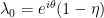
Using

plugging in , and taking logarithms, we get

Now and misses the standard compact set , so since  we have
(since  and is infinitesimal). So we can Taylor expand in about :

Taking expectations and using  ,
,

Plugging in  we see the claim.
I’m not sure who originally came up with the idea to reason like this; I think Tao credits M. J. Miller. Whoever it was had an interesting idea, I think:  is a level set of , but one that a priori doesn’t tell us much about . We have just replaced it with a level set of , a function that is explicitly closely related to , but at the price of an error term.
5. Fine control
We finish this series. If you want, you can let be a standard real. I think, however, that it will be easier to think of as “infinitesimal, but not as infinitesimal as the term of the form o(1)”. In other words,  is smaller than any positive element of the ordered field
  ; briefly, is infinitesimal with respect to . We still reserve to mean an infinitesimal with respect to . Now
  by underspill, since this is already true if is standard and
  . Underspill can also be used to transfer facts at scale to scale . I think you can formalize this notion of “iterated infinitesimals” by taking an iterated ultrapower of
  in the theory of ordered rings.
Let us first bound  . Recall that
  so
so  but in fact we can get a sharper bound. Since is discrete we can get
  arbitrarily close to whatever we want, say
  or
or  . This will give us bounds on
  when we take the Taylor expansion

Lemma 8 Let  be standard. Then

Proof: Let be a standard compact set which misses and a zero of . Since  (since is close to ) and
  has positive standard part (since
  ) we can take Taylor expansions

and

in about  . Taking expectations we have

and similarly for . Thus

since

Since
we have

Now  so
so  , whence

Now recall that is uniformly distributed on , so we can choose  so that
Thus
which we can plug in to get the claim.
Now we prove the first part of the fine control lemma.
Lemma 9 One has

Proof: Let ![{\theta_+ \in [0.98\pi, 0.99\pi],\theta_- \in [1.01\pi, 1.02\pi]}](https://s0.wp.com/latex.php?latex=%7B%5Ctheta_%2B+%5Cin+%5B0.98%5Cpi%2C+0.99%5Cpi%5D%2C%5Ctheta_-+%5Cin+%5B1.01%5Cpi%2C+1.02%5Cpi%5D%7D&bg=ffffff&fg=000000&s=0&c=20201002) be standard reals such that
be standard reals such that  . I don’t think the constants here actually matter; we just need
  or something. Anyways, summing up two copies of the inequality from the previous lemma with
  we have

since

That is,

Indeed,

so

If we square the tautology  then we get

Taking expected values we get

or in other words

where we used the Taylor expansion
obtained by Taylor expanding  about and applying
  . Using
we get
Thus

Dividing both sides by ![{1 + \frac{1}{1.9 + o(1)} + o(1) \in [1, 2]}](https://s0.wp.com/latex.php?latex=%7B1+%2B+%5Cfrac%7B1%7D%7B1.9+%2B+o%281%29%7D+%2B+o%281%29+%5Cin+%5B1%2C+2%5D%7D&bg=ffffff&fg=000000&s=0&c=20201002) we have
we have

In particular

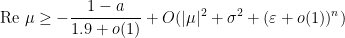
Now we treat the imaginary part of  . The previous lemma gave

Writing everything in terms of real and imaginary parts we can expand out

Using the bounds

(Which follow from the previous paragraph and the bound  ), we have

Since is discrete we can find  arbitrarily close to
  which meets the hypotheses of the above equation. Therefore

Pkugging everything in, we get

Now  since is infinitesimal; therefore we can discard that term.
Now we are ready to prove the second part. The point is that we are ready to dispose of the semi-infinitesimal . Doing so puts a lower bound on  .
.
Lemma 10 Let 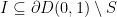 be a standard compact set. Then for every
  ,
,

Proof: Since is uniformly distributed on , there is a zero of with 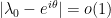 . Since , we can find an infinitesimal
  such that
and  . In the previous section we proved

Using  and plugging in we have

Now
Taking expectations,

Taking a Taylor expansion,

so by Fubini’s theorem

using the previous lemma and  we get

We also have

since is deterministic (and  , and
, and  ; very easy to check!) I think Tao makes a typo here, referring to
  , which seems irrelevant. We do have

since  . Plugging in
we get

I think Tao makes another typo, dropping the Big O, but anyways,

so by the triangle inequality

By underspill, then, we can take  .
.
We need a result from complex analysis called Jensen’s formula which I hadn’t heard of before.
Theorem 11 (Jensen’s formula) Let  be a holomorphic function with zeroes
  and
and  . Then

In hindsight this is kinda trivial but I never realized it. In fact  is subharmonic and in fact its Laplacian is exactly a linear combination of delta functions at each of the zeroes of
  . If you subtract those away then this is just the mean-value property

Let us finally prove the final part. In what follows, implied constants are allowed to depend on  but not on
  .
.
Lemma 12 For any standard  ,
,

Besides,
Proof: Let be the Haar measure on . We first prove this when  . Since is discrete and is compact, for any standard (or semi-infinitesimal)
  , there is a standard compact set

such that
By the previous lemma, if then

and the same holds when we average in Haar measure:

We have

so, using the Cauchy-Schwarz inequality, one has

Meanwhile, if  then the fact that
implies

and hence

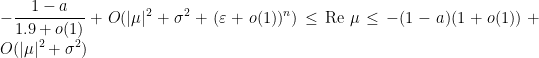
We combine these into the unified estimate

valid for all  , hence almost surely. Taking expected values we get

In the last lemma we bounded  so we can absorb all the terms with in them to get

We also have

(here Tao refers to a mysterious undefined measure  but I’m pretty sure he means ). Putting these integrals together with the integrals over
  ,
,

By underspill we can delete , thus

We now consider the specific case  . Then

Now Tao claims and doesn’t prove

To see this, we expand as

using Fubini’s theorem. Now we use Jensen’s formula with  , which has a zero exactly at . This seems problematic if
  , but we can condition on
  . Indeed, if then we have
which already gives us what we want. Anyways, if , then by Jensen’s formula,

So that’s how it is. Thus we have
Since  ,
,  , so the same is true of its expected value
  . This gives the desired bound
We can use that bound to discard from the average

thus

Repeating the Jensen’s formula argument from above we see that we can replace with  for any
  . So this holds even if is not necessarily nonnegative.
 , namely the fact that every linear operator has an eigenvalue, that every linear operator has a unique Jordan canonical form, and the Cayley-Hamilton theorem. In all of these cases, one could prove the theorem using determinants, but there’s no good reason to, since there is a perfectly reasonable structure theory of linear operators over
  , which is the case for most of the results in the latter half of the book, except for one single chapter about the structure theory over
  . But I do think that a lot of the angry comments I’ve seen about the book on Reddit and elsewhere, which mainly focus on the issue of determinants, are just totally out to lunch.)
 of the linear operator T acting on a vector space V of dimension n, which is a rational map from
  to a space of matrices. Clearly an eigenvalue is a pole of R, and the number of poles equals the number of zeroes (this is clearly true when
  , T must have n eigenvalues. (If
  counted with multiplicity. If
  around the puncture of
  and define
  and similarly
  It is now a straightforward consequence of Cauchy’s integral formula that
  is nilpotent and we have
  . Furthermore, if
  is the image of
  , then A acts on
  , and we have a direct sum decomposition
  . That implies that
  , and replacing the differential form
  with some sort of algebraic analogue of cohomology.
 . This argument ostensibly works over
  where Y is a compact Hausdorff space. By Alexandroff’s theorem, X always has a compactification, but in general if X is not compact then X may have multiple compactifications. We consider the category Comp X of compactifications of X equipped with continuous surjections which preserve X; the Alexandroff compactification is the final object of Comp X.
 where
where  is the Banach space of bounded continuous functions on X with its supremum norm, and the functor Spec is taken in the sense of C*-algebras (thus Spec A consists of maximal closed ideals equipped with the Zariski-Jacobson topology). This proof is presumably inoffensive to anyone who accepts ZFC (and offensive to anyone who does not, since one needs Zorn’s lemma to show that
  is a morphism in Comp X, then since X is dense in Z, the underlying continuous surjection
  be a chain in Comp X; then
  . Since
  is a compact Hausdorff space by Tychonoff’s theorem, so is C. Taking the inverse limits of the open dense embeddings
  , we obtain an open dense embedding
  , so C is an upper bound of
  is a large category. To see that Comp X is equivalent to a small category, it suffices to show that there is a cardinal
  such that every compactification of Comp X has at most
  in Comp X, and the set-theoretic rank of Z is at most
  . Furthermore, if Y is a compactification of X and
  , then, since X is dense in Y, by the boolean prime ideal theorem there is an ultrafilter U on the set Open X of open subsets of X such that
  . Since Y is Hausdorff, it follows that y is the UNIQUE limit of U, but some cardinal arithmetic can be used to show that if
  is the cardinality of X, then there are only
  ultrafilters on Open X (since elements of an ultrafilter on Open X are open subsets of X), so the cardinality of Y is at most
  .
. be a regular cardinal. We say that
  is an inaccessible cardinal if for every cardinal
  ,
,  . We say that
  such that
  .
. . Then there are inaccessible cardinals
  . If
. If  and Y is a compactification of X, then Y can be obtained as an extension of the Alexandroff compactification by splitting nets, but
  . Therefore
  is a small category in
  , so X has a Stone–Čech compactification
  with
with  .
. is by definition a smooth function on the cotangent bundle of X (for which certain seminorms are finite). This was curious to me — you can motivate it by saying that a symbol is an observable and the cotangent bundle is “phase space” in the sense that a point
  consists of a position x and a momentum
  , but why should the momentum live in a cotangent space and not the fiber of some other vector bundle? When we quantize a symbol a, defining an operator a(D) by formally substituting the differential operator
  in place of the momentum, we by definition obtain a pseudodifferential operator. Now let
  be a diffeomorphism, and introduce the pushforward symbol
  . This is the “right” definition in the sense that
  .
. modulo symbols of order m – 1. But
  is invariantly defined as an isomorphism of tangent bundles
  , so its transpose should be an isomorphism
  of the dual bundle. This only makes sense if
  is a covector at y.
 on Y, then the operator
  is a pseudodifferential operator on Y (in the sense that it is the quantization of a symbol on Y; here the pushforward
  is defined to be the inverse of the pullback
  ). Since Y is an open subset of
  . However, in geometry one frequently has to deal with sections of more general vector bundles over M. For example, a 1-form is a section of the cotangent bundle. If E, F are vector bundles over M of rank r, s respectively, one may define the Hom-bundle Hom(E, F), which locally is isomorphic to the matrix bundle
  . Then a pseudodifferential operator from sections of E to sections of F is nothing more than a linear map which, after trivialization of E and F, looks like a $s \times r$ matrix of pseudodifferential operators on M. The principal symbol of such an operator sends the cotangent bundle of M into the Hom-bundle Hom(E, F).
 of pseudodifferential operators of order
  , this assumption is no loss of generality. Under this assumption, the top-order term of a symbol — that is, the principal symbol — satisfies the pushforward formula
  (here
(here  is the
  th symbol class). The principal symbol encodes important information about the nature of the operator; for example we have:
 near infinity of each cotangent space.
 . For example the Laplace-Beltrami operator is elliptic on Riemannian manifolds since its symbol is
  ; since the quadratic form induced by a Lorentzian metric is not positive-definite, it follows that on Lorentzian manifolds, the Laplace-Beltrami operator is not elliptic. Since a Lorentzian Laplace-Beltrami operator is really just the d’Alembertian, whose symbol is
  , this should be no surprise.
 if there is a conic neighborhood of
  wherein
  near infinity. Otherwise, we say that
  if in a neighborhood of x, A is elliptic when restricted to the direction
  .
. , and its projection to M is exactly the singular support ss(u). Indeed,
  iff for every pseudodifferential operator A in a sufficiently small neighborhood of x,
  can be made smooth is by cutting off u to away from
  , which can be done by pseudodifferential operators of order 0 which are elliptic in the x-direction, but not possibly in the y-direction, along the x-axis.
 . Let us therefore begin by studying the “pseudotransport” equation
  .
. is uniformly bounded in
  and continuous in
  , and the real part of a is uniformly bounded from below. Then we have the energy estimate
 and
and  we can find
  which solves the pseudotransport equation. In particular, given Schwartz initial data, it follows that u is smooth.
 and assume that the principal symbol exists and is imaginary. (This forces the transport operator to be real and of order 1.) Let q be a symbol of order 0 on space, with principal symbol
  . If in fact Q(D) is a pseudodifferential operator on spacetime such that such at time 0, Q(0) = q, and Q(t, D) commutes with
  then Qu solves the pseudotransport equation. (Actually, we will find Q so that
 ![[Q(t), \partial_t + a(t, x, D_x)]](https://s0.wp.com/latex.php?latex=%5BQ%28t%29%2C+%5Cpartial_t+%2B+a%28t%2C+x%2C+D_x%29%5D&bg=ffffff&fg=000000&s=0&c=20201002) is a pseudodifferential operator of order
is a pseudodifferential operator of order  then WF(u) is contained in Char Q, and WF(u) should be the intersection of all such sets Char Q.
 be the principal symbol of a(D) and suppose that
  , where
  is principal, is given. Then the principal symbol of
 ![[\partial_t + a(t, x, D_x), Q(t, x, D)]](https://s0.wp.com/latex.php?latex=%5B%5Cpartial_t+%2B+a%28t%2C+x%2C+D_x%29%2C+Q%28t%2C+x%2C+D%29%5D&bg=ffffff&fg=000000&s=0&c=20201002) is the Poisson bracket
is the Poisson bracket
 is the Hamilton vector field of a symbol p. By inducting on j, we can use this computation to compute
  and conclude that modulo an error term of order
  given by the Hamiltonian
  . That is, if
  , then
  . This result is a sort of “propagation of singularities” for the pseudotransport equation, which generalizes the fact that the transport equation acts on Dirac masses by transporting them, as expected.
 that is a “time coordinate”. The level surfaces of
  and
and  denote the present and future, respectively.
 and for every
  such that
  , there are m distinct
  such that
  .
. with its usual Riemannian metric and
  we can find exactly m real numbers
  such that
  . In the case of the d’Alembertian, we have
  , and indeed given
  .
. , let v be a vector field such that
  , so v points “forward in time”. The action of v is “differentiating with respect to time”. Note that this hypothesis prevents
  . Assume we are given an inhomogeneous term
  satisfying
  and initial data
  , j < m. Then there is
  supported in
  such that Pu = f in
  and
and  in
in  .
. .
. induces a flow on
  which preserves q.
 . A bicharacteristic of Q is an orbit of the bicharacteristic flow.
 where
where  ranges over all multiindices of order m and
  . In order that the characteristic variety of Q have more than one real point, there must be some
  positive and some negative. But this is exactly the situation of the d’Alembertian, whose principal symbol is
  .
. . Let P be a pseudodifferential operator of real principal symbol p and order m.
 , if
, if  , then
  are linearly independent at
  .
. of
of  , there is T < 0 such that for every
  ,
,  and
and  .
. is an error term created by the use of pseudodifferential operators and is not interesting. The operator
  is a cutoff which microlocalizes the problem to a neighborhood to the conic set U. We are interested in WF(u) – WF(f), so we want
  and
and  . Actually, since we only care about the complement of WF(f), we might as well take f Schwartz, in which case we can take
  and simplify the propagation estimate to
 , then
  , but we assumed f Schwartz, so this implies
  , so that if we traveled back along the bicharacteristic flow
  with T < 0.
 is a
is a  invertible matrix, then the determinant of A is either positive, in which case we say it is orientation-preserving, or negative, in which we case we say it is orientation-reversing. A change of coordinates is said to be orientation-preserving (resp. reversing) if its Jacobian matrix is orientation-preserving (resp. reversing). Thus on an orientable manifold there exist two possible orientations — in the low-dimensional cases, right and left, clockwise and counterclockwise, and right-handed and left-handed.
 . The trouble is that angular momentum of a particle rotating in positive orientation is by definition positive, so one first needs to decide what one means by positive orientation.
 to its “topological index”, which is a rational number defined in terms of the cohomology of
  . This would entirely be for fun, and I may blog about it, so as to tell the story of a hapless analyst faffing around hopelessly in deep algebra.
 .
. , references to which we will suppress when possible. Let

 is a fine sheaf, i.e. it has partitions of unity subordinate to every open cover, then
  and the long exact sequence collapses to the exact sequence
 induces a bounded linear map
  such that
  is the kernel of
  is the cokernel of
  satisfies
 denote the sheaf of holomorphic functions on
  the Cauchy-Riemann operator. Let
  denote the sheaf of smooth functions on
  , for
, for  open, induces a short exact sequence of sheaves of Fréchet spaces

 is by definition the genus
 on
on  norm on
 clashes with the notation for cohomology, so let me use
  to denote the completion of
 ranges over multiindices. Then
  and
and  . The kernel of
  , by Liouville’s theorem and Weyl’s lemma), so to deduce that
 which satisfy
  . By definition of the Sobolev norm, we have
 is smooth. Then we can write
  where
where  and
and  are holomorphic. In particular,
  and
and  , so
, so
 . Taking a Cauchy estimate, we see that

 be a sequence in
  with
with  , and assume that the
  are Cauchy in
  . Without loss of generality we may assume that
  where
where  , and thus assume that they are in fact bounded. By the Rellich-Kondrachov theorem (which says that the natural map
 , hence the
  . Therefore
  has no boundary implies that for any
  ,
,
 . Since
  is closed, the dual of the cokernel of
  ; by the Rellich-Kondrachov theorem, the unit ball of
  be a polynomial over
  of degree
  . Then the equation
  has
has  , counting multiplicity.
 is a real closed field, but since there are lots of real closed fields, one usually defines
  such that
  does not have a square root in
  . As usual, we want to show that
  is constant.
 is finite. Therefore
  , by stereographic projection. Also by stereographic projection, one can cover the sphere by two copies of
  , one centered at the south pole that misses only the north pole, and one centered at the north pole that only misses the south pole. Thus one can define the Laplacian,
  , in each of these coordinates; it remains well-defined on the overlaps of the charts, so
  is well-defined on all of
  . (In fancy terminology, which may help people who already know ten different proofs of the fundamental theorem of algebra but will not enlighten anyone else, we view
  is called harmonic provided that
  . We claim that
  where
where  . Then
  exactly if