Hausdorff dimension of families of sets via algorithmic randomness

A rather annoying fact about Hausdorff dimension is that, if one has a family $X_t$ of sets parametrized by $t \in T$ , then it is typically not true, or at least not easy to show, that the Hausdorff dimension of $\bigcup_{t \in T} X_t$ is $\dim T + \sup_{t \in T} \dim X_t$ , as one would expect from, say, algebraic geometry. For example, if $X, Y$ are Borel sets, then it is not necessarily true that $\dim(X + Y) = \dim X + \dim Y$ . When one goes a bit beyond the Borel sets (and does not assume the existence of large cardinals), things get much more ridiculous, and in fact there can exist a coanalytic set of full dimension whose closed subsets are all countable.

I ran into this issue recently, when I needed the following theorem to be true:

Theorem. Let $\|\cdot\|$ be an asymmetric norm on $\mathbf R^n$ , let $V$ be a subset of the unit sphere of the dual norm of $\|\cdot\|$ , and let $S = \bigcup_{v \in V} v^*$ .
Then

$\displaystyle \dim S \leq \dim V + \sup_{v \in V} \dim(v^*)$ .

Here, $v^* := \{x \in \mathbf R^n: \langle v, x\rangle = \|x\| = 1\}$ is the dual flat of $v$ .

The techniques used to prove this theorem have nothing to do with the problem I am working on, and I think it is an instructive example of how they are used; so I record the theorem here, rather than in the paper I am writing.

Specifically, the theorem shall be proven using algorithmic randomness, following the framework of Algorithmic information, plane Kakeya, and conditional dimension. We recall this framework here.

Let $\Sigma$ be the set of all finite binary strings. If $\sigma, \sigma' \in \Sigma$ , we write $\sigma \frown \sigma'$ for their concatenation. We write $|\sigma|$ for the length of $\sigma$ .

A set $\Gamma \subset \Sigma$ is prefix-free if for every $\sigma, \sigma' \in \Gamma$ and $\tau \in \Sigma$ , if $\sigma \frown \tau = \sigma'$ , then $|\tau| = 0$ . By standard coding techniques one can represent points in $\mathbf Q^n$ or $\mathbf N$ as finite binary strings, in such a way that the set of binary strings which are used to code points in $\mathbf Q^n$ or $\mathbf N$ is prefix-free; we shall exploit this fact without comment.

A function $f: \mathrm{dom}(f) \to \Sigma$ is partial computable if $\mathrm{dom}(f) \subseteq \Sigma$ and there exists a Turing machine $\Phi$ such that for every binary string $\sigma$ , $\sigma \in \mathrm{dom}(f)$ iff $\Phi$ halts with input $\sigma$ , and if $\sigma \in \mathrm{dom}(f)$ , then $\Phi$ prints $f(\sigma)$ . A partial computable function $f$ is prefix-free if $\mathrm{dom}(f)$ is prefix-free. A prefix-free function $U$ is universal if for every prefix-free partial computable function $f$ , there exists $\rho_f \in \Sigma$ such that $\{\rho_f: f \text{ is a prefix-free function}\}$ is prefix-free, and for every $\sigma \in \mathrm{dom}(f)$ , $U(\rho_f \frown \sigma) = f(\sigma)$ . Thus $U$ is playing the role of a “compiler”. There exists a universal prefix-free function $U$ ; we fix one, once and for all. If $f$ is prefix-free and $\rho_f$ is chosen so that $f(\sigma) = U(\rho_f \frown \sigma)$ , then $\rho_f$ is a program which computes $f$ .

The Kolmogorov complexity of $\sigma \in \Sigma$ is

$\displaystyle K(\sigma) := \min \{|\rho|: U(\rho) = \sigma\}$ .

Since we can code rational points, or integers, as binary strings, it makes sense to take their Kolmogorov complexities. For any $j \in \mathbf N$ , the program which simply decodes the binary expansion of $j$ provides an upper bound on $K(j)$ , namely $K(j) \leq \log j + O(1)$ (where logarithms are base- $2$ ). Given $x \in \mathbf R^n$ and $r \geq 0$ , the Kolmogorov complexity of $x$ to $r$ bits is

$\displaystyle K_r(x) := \inf \{K(q): q \in \mathbf Q^n \cap B(x, 2^{-r})\}$ .

The effective Hausdorff dimension of $x$ is

$\displaystyle \dim(x) := \liminf_{r \to \infty} \frac{K_r(x)}{r}$ .

It can be shown that $\dim(x)$ does not depend on the choice of the universal function $U$ .

The above concepts can be relativized. Let $A \subseteq \Sigma$ , and in the above definitions, replace “Turing machine” with “Turing machine with oracle $A$ .” Let $K_r^A(x)$ and $\dim^A(x)$ denote the Kolmogorov complexity and effective Hausdorff dimension of $x \in \mathbf R^n$ measured with oracle $A$ .

The key theorem, which interprets Hausdorff dimension as a measure of indescribability, and is proven in Plane Kakeya… is,

Point-to-set principle. For every set $E \subseteq \mathbf R^n$ ,

$\displaystyle \dim E = \min_{A \subseteq \Sigma} \sup_{x \in E} \dim^A(x)$ .

In particular, for each set $E \subseteq \mathbf R^n$ , there exists an oracle $A_E \subseteq \Sigma$ such that if $A \geq_T A_E$ then $\dim E = \sup_{x \in E} \dim^A(x)$ . The oracle $A_E$ is called a Hausdorff oracle for $E$ .

Lemma 1. Let $X$ be a compact convex subset of $\mathbf R^n$ , and assume $s := \dim X \leq n - 1$ .
There exists $C \geq 1$ such that for every $h > 0$ , with $X_h := \{x \in \mathbf R^n: \mathrm{dist}(x, X) < h\}$ ,

$\displaystyle C^{-1} h^{n - s} \leq \mathrm{vol}(X_h) \leq Ch^{n - s}$ .

To prove the lemma, observe that since $s \leq n - 1$ , $X$ has empty interior. Since $X$ is convex, it follows that $X$ is contained in an $n - 1$ -plane $P$ . If $s \leq n - 2$ , then it is enough to prove the theorem with $\mathbf R^n$ replaced by $P$ , so we may use induction on $n - s$ to reduce to the case that $s = n - 1$ .

If $s = n - 1$ , then $X$ has nonempty interior in $P$ , so $X$ contains a ball $Y$ in $P$ , and (viewing $Y$ as a subset of $\mathbf R^n$ ) $Y_h$ is a cylinder of length $h$ , so $\mathrm{vol}(X_h) \geq \mathrm{vol}(Y_h) \gtrsim h$ . Conversely, since $X$ is compact, $X$ is contained in a ball $Z$ in $P$ , and the converse inequality holds, proving the lemma.

Lemma 2. Let $\|\cdot\|$ be an asymmetric norm on $\mathbf R^n$ . Then there exists $C > 0$ such that for each point $v$ on the unit sphere of the dual norm of $\|\cdot\|$ , and each $x \in \mathbf R^n$ ,

$\displaystyle \mathrm{dist}(x, v^*) \leq C(|\|x\| - 1| + |\langle v, x\rangle - 1|)$ .

This is just some linear algebra, and comparability of norms, so I’ll leave out the proof of this lemma.

Now to prove the main theorem. By the point-to-set principle, we may choose a Hausdorff oracle $A_V$ for $V$ . By rounding off $\|x\|$ to a suitable rational number for each $x \in \mathbf R^n$ , we may find a function $\psi: \mathbf Q^n \times \mathbf N \to \mathbf Q_+$ such that for each $q \in \mathbf Q^n$ and $r \geq 0$ , $|\psi(q, r) - \|q\|| < 2^{-r}$ . Then there is an oracle $A_\psi$ which computes $\psi$ ; let $A := A_\psi \oplus A_V$ .

For each $v \in V$ and $r \in \mathbf N$ , choose $v_r \in 2^{-r} \mathbf Z^n$ such that $|v - v_r| < \sqrt n/2^r$ and $K(v_r) \leq K_r(v) + O(1)$ . By comparability of norms, there exists $R \in \mathbf N$ such that for every $v, r, q$ , if $|\langle v_r, q\rangle - 1| + |\psi(q, r) - 1| \leq 1$ , then $q \in [-R, R]^n$ . So $2^{-r} \mathbf Z^n \cap [-R, R]^n$ is a finite set and therefore the function $f_{v, r}: \mathbf N \to 2^{-r} \mathbf Z^n$ which returns the lexicographically $j$ th $q \in 2^{-r} \mathbf Z^n$ such that $|\langle v_r, q\rangle - 1| + |\psi(q, r) - 1| < 2^{-(r-3)}$ , and returns $0$ if no such point exists, is well-defined.

Fix $v \in V$ and $r \in \mathbf N$ , and define the following algorithm which takes input $j$ , and uses $A$ as an oracle:

Let $i := 1$ .
For each in lexicographic order:
1. If $|\langle v_r, q\rangle - 1| + |\psi(q, r) - 1| < 2^{-(r-3)}$ , increment $i$ .
2. If $i = j$ , return $q$ .
Return $0$ .

Thus this algorithm computes $f_{v, r}$ , so for any $j$ such that $f_{v, r}(j) \neq 0$ ,

$\displaystyle K^A(f_{v, r}(j)) \leq K^A(v_r) + K(r) + K(j) + O(1)$ .

For each $x \in v^*$ , choose $x_r \in 2^{-r} \mathbf Z^n$ such that $|x - x_r| < \sqrt n/2^r$ . Then, if $r \geq \log n/2$ , one can check that

$\displaystyle |\langle v_r, x_r\rangle - 1| + |\psi(x_r, r) - 1| < 2^{-(r - 3)}$ ,

which establishes that there exists $j \in \mathbf N$ such that $x_r = f_{v, r}(j)$ . In particular, with $r_0 := \lceil \log n/2\rceil$ ,

$\displaystyle K_{r - r_0}^A(x) \leq K_r^A(v) + \log j + O(\log r)$ .

It remains to estimate $j$ , but by Lemma 2, there exists $r_1 \in \mathbf N$ which only depends on $\|\cdot\|$ , such that for every $j$ such that $f_{v, r}(j) \neq 0$ , $\mathrm{dist}(f_{v, r}(j), v^*) \leq 2^{-(r - r_1)}$ . Let $U := \{\mathrm{dist}(\cdot, v^*) < 2^{-(r - r_1 - 1)}\}$ , $j_0$ the largest $j$ such that $f_{v, r}(j) \neq 0$ , and $s := \dim(v^*)$ , so by Lemma 1, $\mathrm{vol}(U) \lesssim 2^{-r(n - s)}$ ; for any $j \leq j_0$ , $B(f_{v, r}(j), 2^{-r}) \subseteq U$ ; and for any $y \in U$ , $\mathrm{card} \{j \in J: |f_{v, r}(j) - y| < 2^{-r}\} \leq 2^n$ . Combining these facts, we see that

$\displaystyle \sum_{j=1}^{j_0} \mathrm{vol}(B(f_{v, r}(j), 2^{-r})) \leq 2^n \mathrm{vol}(U) \lesssim 2^{-r(n - s)}$

and therefore, since each ball has volume $\sim 2^{-rn}$ , $j_0 \lesssim 2^{rs}$ . From this, one can show that

$\displaystyle K_{r - r_0}^A(x) \leq r(\dim V + \dim(v^*)) + O(\log r)$ .

The theorem now follows from the point-to-set principle.

Dupin’s theorem in general dimension

Let $d \geq 3$ . We say that two smooth foliations F, G of codimension 1 in $\mathbb R^d$ are orthogonal if for any $p \in \mathbb R^d$ , the leaves X, Y of F, G passing through p are orthogonal at p.

Dupin’s theorem. Let $\vec F = (F_1, \dots, F_d)$ be a d-tuple of mutually orthogonal foliations of codimension 1 in $\mathbb R^d$ . Let $p \in \mathbb R^d$ , let $X_i$ denote the leaf of $F_i$ passing through p, and let
$Y_i := \bigcap_{j \neq i} X_j$ . Then $Y_i$ is tangent to a principal curvature vector of $X_j$ at p whenever $i \neq j$ .

This theorem is well-known in dimension $d = 3$ , but it was brought to my attention by Hyunwoo Kwon that there does not seem to be a good reference if $d \geq 4$ . This appears to be for superficial reasons: the usual proof is based on properties of the cross product which clearly only hold when $d = 3$ . I call this a superficial reason, because we can easily replace the cross product with the wedge product, and then the argument will work in general. In this blog post, I will record the proof which works for any dimension $d \geq 3$ . (Actually, it works in case $d \leq 2$ as well, but Dupin’s theorem is vacuously true in that case.)

We first check that the conclusion of the theorem makes sense. In fact, $Y_i$ is the intersection of $d - 1$ smooth hypersurfaces, each of which are mutually orthogonal and therefore are transverse. So $Y_i$ is a smooth curve, and its tangent space at p is a line.

Near p, we can find a coordinate system $\vec \xi = (\xi^1, \dots, \xi^d)$ such that the level sets of $\xi^i$ are the leaves of $F_i$ . Let g be the euclidean metric tensor written in the coordinates $\vec \xi$ . Orthogonality of $F_i$ and $F_j$ means that $\langle d\xi^i, d\xi^j\rangle = 0$ . Therefore the cometric

$\displaystyle g^{ij} = \frac{\partial \xi^i}{\partial x^\mu} \frac{\partial \xi^j}{\partial x^\nu} \delta^{\mu \nu}$

is diagonal; therefore the same holds for the metric

$\displaystyle g_{ij} = \frac{\partial x^\mu}{\partial \xi^i} \frac{\partial x^\nu}{\partial \xi^j} \delta_{\mu \nu}$ .

Let (i, j, k) be a distinct triple. Differentiating the equation $g_{ij} = 0$ , we obtain

$\displaystyle 0 = \frac{\partial^2 x^\mu}{\partial \xi^i \partial \xi^k} \frac{\partial x^\nu}{\partial \xi^j} \delta_{\mu \nu} + \frac{\partial x^\mu}{\partial \xi^i} \frac{\partial^2 x^\nu}{\partial \xi^j \partial \xi^k} \delta_{\mu \nu}.$

Thus if we set

$\displaystyle a_{ijk} := \frac{\partial^2 x^\mu}{\partial \xi^i \partial \xi^j} \frac{\partial x^\nu}{\partial \xi^k} \delta_{\mu \nu}$

then we have the system of equations $a_{ijk} + a_{ikj} = 0$ , $a_{jik} + a_{jki} = 0$ , $a_{kij} + a_{kji} = 0$ , $a_{ijk} - a_{jik} = 0$ , $a_{ikj} - a_{kij} = 0$ , $a_{jki} - a_{kji} = 0$ . Here, the first three equations arise from the formula for the differentiated metric and the last three originate from symmetry of second partial derivatives. The only solution of this system of this equation is $a_{ijk} = 0$ for every distinct triple (i, j, k), or in other words

$\displaystyle 0 = \frac{\partial^2 x^\mu}{\partial \xi^i \partial \xi^j} \frac{\partial x^\nu}{\partial \xi^k} \delta_{\mu \nu}$ .

Combining this equation with the equation $g_{ij} = 0$ and the formula for the metric, we see that every vector in the list

$\displaystyle L := \left(\frac{\partial^2 \vec x}{\partial \xi^i \partial \xi^j}, \frac{\partial \vec x}{\partial \xi^1}, \dots, \widehat{\frac{\partial \vec x}{\partial \xi^k}}, \dots, \frac{\partial \vec x}{\partial \xi^d}\right)$

(where the roof means to remove that entry from the list) is orthogonal to $\partial \vec x/\partial \xi^k$ . Therefore every vector in L is contained in a vector space of dimension $d - 1$ , but the length of L is d, so L is linearly dependent.

Let $A_{(k)}$ be the second fundamental form of $X_k$ , written in the coordinate system

$\displaystyle \vec \xi_k := (\xi^1, \dots, \widehat{\xi^k}, \dots, \xi^d)$ .

Then $A_{(k)ij}$ is equal to a scalar times the Hodge star of the wedge product of all of the vectors in L. Since the wedge product of L vanishes, so does $A_{(k)ij}$ , so $A_{(k)}$ is diagonal. Since the metric $h_{(k)}$ on $X_k$ is given by $h_{(k)ij} = g_{ij}$ , $h_{(k)}$ is also diagonal in the coordinate system $\vec \xi_k$ .

It follows that $\partial_{\xi_i}$ is a principal curvature vector of $X_k$ whenever $i \neq k$ . But $\partial_{\xi_i}$ is normal to $X_i$ , so it is tangent to the curve $Y_i$ , as desired.

Finite elements for the highbrow mathematician

In recent years, study of the finite element method for numerically solving PDE has taken an increasingly homological turn. However, at least in my circles, “pure” mathematicians have largely not taken notice of this trend. I suspect that there’s an opportunity for a mutually beneficially partnership here — and so I shall here try to translate some of the ideas of the FEM to the language spoken by pure mathematicians.

The Dirichlet Laplacian, and the basic idea. Let $Pu = f$ be a partial differential equation, which for simplicity I will take to be a linear, elliptic equation of second order with homogeneous Dirichlet data on a compact polytope $\Omega$ . The canonical example is that P is the Laplacian, and then this system reads

$\displaystyle \begin{cases} -\Delta u = f \\ u|_{\partial \Omega} = 0 \end{cases}$

The key thing to observe is that since P is differential, it is local: we can determine $Pu(x)$ from the germ of u at x. Motivated by this observation, we divide and conquer by fixing a family $\mathcal T_h$ of partitions of $\Omega$ into simplices, where each simplex in $\mathcal T_h$ has edge lengths comparable to h. We then fix the space $V_h$ of PL shape functions, which are continuous functions on $\Omega$ whose restriction to each simplex is a linear polynomial. This is a finite-dimensional, hence closed, subspace of the Sobolev space $W^{1, 2}_0(\Omega)$ . Of course, other Sobolev spaces admit better choices of shape functions, which in some cases can be easily read off of the Sobolev embedding theorem.

We now take the orthogonal projection of the equation $Pu = f$ to $V_h$ to obtain a new equation $P_h u_h = f_h$ . If we can solve this equation, then by the orthogonality of the projection, the Bramble-Hilbert lemma for Sobolev spaces, and elliptic regularity, we will have

$\displaystyle \|u - u_h\|_{W^{1, 2}} \lesssim h \|u\|_{\dot W^{2, 2}} \lesssim h \|f\|_{L^2}$

thus for $h \ll 1$ we have a good solution in $W^{1, 2}$ . By modifying the choice of Sobolev spaces and shape functions we can obtain bounds at other regularities.

There are three obstructions to the ability to invert a matrix $P_h$ in a practical amount of time, however:

Unisolvence. The matrix must be square. This is no issue for the Laplacian, since $P_h: V_h \to V_h$ .
Conditioning. The size of the smallest eigenvalue must be bounded from below (so the matrix is not too close to a singular matrix). The smallest eigenvalue $\lambda_{1, h}$ of $P_h$ is controlled from below by the Dirichlet spectral gap of $\Omega$ , which is bounded from below as long as $\Omega$ is not too fractalline or degenerate:
$\displaystyle |\lambda_{1, h}| \gtrsim |\lambda_1| \gtrsim 1$ .
Sparsity. Most of the entries of $P_h$ should be zero, and the nonzero entries should be easy to pick out, so that we don’t have to iterate over the whole matrix when we invert it. This is ensured by locality: if $(i, j)$ is a pair of indices corresponding to a shape function on a simplex K, then the only nonzero entries in row i or column j are for shape functions on simplices which are adjacent to K.

Elliptic Maxwell, and dealing with systems. Unfortunately the Laplacian is positive-definite, not a system, and otherwise generally just about the nicest PDE there is. We want to solve other PDE, too, and they will probably be of greater interest.

So let us consider the Maxwell equations. They are hyperbolic, however, and this adds a lot of complications outside the scope of this blog post. So we assume time-independence, and in that case the Maxwell equations decouple into two elliptic systems: the electric and magnetic systems. The electric system can be rewritten as the Laplacian, so we focus on the magnetic system

$\displaystyle \begin{cases} \nabla \cdot B = 0 \\ \nabla \times B = J \\ B|_{\partial \Omega} \cdot \vec n_\Omega = 0 \end{cases}$

where B is the magnetic field, $\vec n_\Omega$ is the normal field to $\partial \Omega$ , and the electric current J is given. The right-hand side of the equation $\nabla \cdot B = 0$ is not data, so that zero is not secretly an epsilon: it asserts that B has no monopoles. Therefore it is natural to place B in a space of divergence-free vector fields. Doing so will impose that $\nabla \cdot B = 0$ as opposed to simply $\|\nabla \cdot B\|_{L^2} \ll 1$ or a similar “approximate monopole inequality”. I will refer to such a B as divergence conforming; a similar condition appears when one tries to solve the Stokes or Navier-Stokes equations for a liquid.

This can be done directly, but we’re going to have to go homological eventually anyways, so let’s rewrite the magnetic Maxwell equations as

$\displaystyle \begin{cases} dB = 0 \\ d * B = * J \\ \iota_{\partial \Omega}^* B = 0 \end{cases}$

where B is now viewed as a 2-form, J is now viewed as a 1-form, and $\iota: \partial \Omega \to \Omega$ is the inclusion map. This interpretation is quite natural, because it views B as something that we want to integrate over a surface $\Sigma$ , so that $\int_\Sigma B$ is now the magnetic flux.

Let $\Omega^\ell$ be the space of $\ell$ -forms, $K^\ell$ the kernel of $d: \Omega^\ell \to \Omega^{\ell + 1}$ , and observe that

$\displaystyle K^2 = d\Omega^1 \oplus H^1(\Omega)$

where the de Rham cohomology $H^1(\Omega)$ is a finite-dimensional space that does not depend on h, so we can solve it separately. So we may assume that $B = dA$ for some 1-form A. Without loss of generality, we may assume that A is in Coulomb gauge, in which case

$\displaystyle \begin{cases} d * dA = J \\ d * A = 0 \\ A|_{\partial \Omega} = 0 \end{cases}$

Here we don’t actually care about the fact that $d * A = 0$ , so if we pick up some numerical error there, it doesn’t matter. After all, we actually care about $dA$ , not A itself, and $dA$ is left invariant by gauge transformations of A.

The Whitney complex. It remains to find suitable shape $\ell$ -forms for all $\ell \in \{0, \dots, 3\}$ . We cannot choose them arbitrarily, however, because we must preserve unisolvence of the maps $d_h: \Omega^\ell \to K^\ell/H^\ell(\Omega)$ . The natural norm to put on $\Omega^\ell$ turns out to be

$\displaystyle \|\varphi\| := \|\varphi\|_{L^2} + \|d\varphi\|_{L^2}$

so that d is continuous and is elliptic modulo its kernel and cokernel. One can then use this fact, plus the theory of Fortin operators, to show that the discrete d on the space of shape forms is well-conditioned.

A natural way to preserve unisolvence is to find a family of morphisms of chain complexes $\Pi_h: \Omega^\bullet \to V_h^\bullet$ where $V_h^\bullet$ is a family of chain complexes associated to the triangulations $\mathcal T_h$ . This was more or less accomplished by Nédélec in the 1980s, but not in this language, and after quite a lot of work. However, the modern viewpoint is that Nédélec forms are nothing more than Whitney forms, which were discovered by Whitney decades prior:

Definition. Let $\sigma$ be a d-simplex, and let C be a simplicial k-chain in $\sigma$ . The Whitney form dual to C is the unique k-form $\varphi$ on $\sigma$ such that:

$\varphi_I$ is a linear function on $\sigma$ for every increasing multiindex I.

If $\iota: \tau \to \sigma$ is a k-face of $\sigma$ , then $(\iota^* \varphi)_I$ is a constant function on $\tau$ for every increasing multiindex I.

If $\iota: \tau \to \sigma$ is a k-face of $\sigma$ , then
$\displaystyle \int_\tau \varphi = \langle C, \tau\rangle$ .

The Whitney complex associated to a triangulation $\mathcal T_h$ is the chain complex of all $L^2$ k-forms $\varphi$ on $\Omega$ , such that:

For every d-simplex $\sigma \in \mathcal T_h$ , $\varphi|_\sigma$ is a Whitney k-form on $\sigma$ .

For every k-face $\iota: \tau \to \Omega$ in $\mathcal T_h$ , the pullback $\iota^* \sigma$ exists in the sense of the Sobolev trace theorem. In particular, there is no jump discontinuity.

The Whitney projection $\Pi_h$ associated to a triangulation $\mathcal T_h$ maps a k-form $\varphi$ to the unique k-form $\Pi_h \varphi$ in the Whitney complex associated to $\mathcal T_h$ such that for every k-face $\tau$ ,

$\displaystyle \int_\tau \Pi_h \varphi = \int_\tau \varphi$ .

See the paper of Dodziuk for more on the construction of Whitney forms. Anyways, we have a version of the Bramble-Hilbert lemma, as proven by Bramble, Falk, and Whinther:

Theorem. For any k-form $\varphi$ ,

$\displaystyle \|(1 - \Pi_h)\varphi\| \lesssim h (\|\varphi\|_{W^{1, 2}} + \|d\varphi\|_{W^{1, 2}})$ .

Putting it all together. To solve the elliptic Maxwell system, we can now proceed as when we solved the Laplacian.
Let $P_h$ be the projection of the matrix of differential operators

$\displaystyle P_h = \begin{bmatrix}d * d \\ d * \end{bmatrix}$

to the first space in the Whitney complex. Then $P_h$ is clearly unisolvent and sparse, and one can show that it is well-conditioned as well. We conclude that we can solve

$\displaystyle P_h A_h = \begin{bmatrix}\Pi_h J \\ 0\end{bmatrix}$

for some 1-form $A_h$ , and then $B_h := dA_h$ satisfies

$\displaystyle \|B_h - B\|_{L^2} \leq \|A - A_h\| \lesssim h(\|A\|_{W^{1, 2}} + \|B\|_{W^{1, 2}})$

by the Bramble-Hilbert lemma. By Ladyzhenskaya’s inequality ad the fact that A is in Coulomb gauge,

$\displaystyle h(\|A\|_{W^{1, 2}} + \|B\|_{W^{1, 2}}) \lesssim h\|B\|_{W^{1, 2}}$

Finally, by elliptic regularity,

$\displaystyle h\|B\|_{W^{1, 2}} \lesssim h\|J\|_{L^2}$

so we conclude

$\displaystyle \|B_h - B\|_{L^2} \lesssim h\|J\|_{L^2}$

and so B is a good approximation to J in $L^2$ , which is in addition divergence conforming.

Numerical constants are not a red flag

I do not understand the Yitang Zhang’s claimed proof of an improvement to the zero-free region of a Dirichlet L-function. That will not stop me from weighing in on some of the discourse I’ve seen around the proof, because let’s be honest, nobody else commenting on the proof, other than experts in hard analytic number theory, has any chance of understanding the proof either. And since Peking University and Nature both have announcements of the proof that are not entirely correct, I can at least promise that what follows will be better than their discussion 🙂

Since the announcement of the proof, several comments on r/math, among other places, have observed how unusual it is that Zhang’s proof contains specific (and, in the minds of the commenters, arbitrary-looking) constants. This seems like the final form of the meme that “real mathematicians don’t work with numbers, only concepts” that one often hears undergraduate math majors repeat, but that is simply not true. Zhang claims an explicit bound on the width of the zero-free region, and while his choice of the exact size of the bound was a little bit arbitrary, this is not entirely unusual. [1] I refer to two papers that I recently read which also have explicit bounds and as such have actual numbers all over the place: Dolgopyat’s method and the fractal uncertainty principle and Efficient algorithms for solving the p-Laplacian in polynomial time. In an upcoming paper that I have with some coauthors, we currently have a bound

$\displaystyle L \leq \max(23000 d^{3/2} c_N^{-3/2}, 80^3 ||\partial^2_{xy} \Phi||_{C^0}^3 c_N^{-3}, (2\theta^2)^{-3/4}, (160c_N^2)^{-3})$

though before submitting for publication we may optimize this estimate a bit to get the constants a bit smaller. If we do, they will definitely look less round and more arbitrary.

Anyways, let’s take a look at Zhang’s paper and see where some of the constants that people seem most suspicious of are coming from. Those constants are on page 10 in the draft that’s currently on the arXiv and are

$\displaystyle \iota_2 = 0.94977 - 1.38995i, ~ \iota_3 = -1.00635 - 0.22789i, ~\iota_4 = -0.68738 + 1.60688i$ .

Where do these “iotas” come from, and where are they going? (This will be a reformatting of a reddit comment I made.)

The key estimate is Proposition 2.5, which bounds a quantity defined on the bottom of page 9. (Don’t ask me what the significance of that quantity is.) By Cauchy’s product inequality

$\displaystyle \alpha \beta \leq \frac{\alpha^2}{2\varepsilon} + \frac{\varepsilon \beta^2}{2}$

he needs to prove (2.32) and (2.33), where (2.32) is an estimate of the form

$\displaystyle \alpha^2 < 0.001aP$

and (2.33) is of the form

$\displaystyle \beta^2 < 3000aP$

for some a, P that are determined elsewhere in the proof. Note that if (2.33) was stronger (smaller constant than 3000) he would not need to have such a strong bound in (2.32). However, on page 100 he proves (2.33) by splitting a sum into a dominant term and a bunch of error terms, and then doing the sloppy thing and showing that each of those error terms is at most 100aP or something like that. The result is that he gets a big constant 3000 at the end.

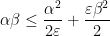
So Zhang needs a small constant in (2.32) to pay for his sloppiness in (2.33) — in other words he needs to choose $\varepsilon$ suitably. Messing around with Cauchy’s product inequality (I did this in desmos), you can convince yourself that the constant in (2.32) can be a little bit bigger than 0.001, but Zhang decided to round down to make the statement of (2.32) less messy.

So now we turn to page 99 to see the proof of (2.32), which comes down to an estimate of the form

$\displaystyle c_1 + c_2 + 2Re(c_3) < 0.001$ .

Here his constant $c_3$ probably easily follows from the iotas, which suggests that he probably made those choices so that 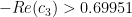$-Re(c_3) > 0.69951$ would be just barely smaller than 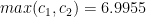$max(c_1, c_2) = 6.9955$ . Those constants are calculated in Sections 8 and 9 respectively. Anyways, since Sections 8 and 9 depend on the iotas as well, it would not be unreasonable to speculate that using some numerical analysis he was able to find that as long as the constants lived in some small ball in the complex plane they would be OK, and then rounded to sufficient precision to obtain the choice of iotas.

I suspect that computing $c_1, c_2$ is probably the hard part of the proof, so I’m not going to try to understand it. However, skimming Sections 8 and 9, it seems like $c_1, c_2$ are obtained by reducing a whole lot of analytic number theory voodoo to the computation of finitely many one-dimensional integrals and then using a computer to evaluate the integrals. This constrains what you can choose the iotas to be, and then by explicit numerical computation one obtains them as given in Section 2.

Zhang’s proof may yet be wrong — and simply because the problem in question is known to be notorious for drawing incorrect proofs (including one due to Zhang himself) — I would be suspicious of any claimed proof until the experts can validate it. However, the fact that he has numerically significant constants in his proof is not a red flag — in fact, since he claims explicit bounds, I would be far more suspicious if this was not true.

[1] One of these days someone is going to write a paper with explicit bounds 69 and 420, and the journal referee will have to decide if this is too unprofessional to publish.

What is the metaverse, and of what use is it?

I am not aware of a consensus on the answer to the titular questions. This is in part because no man is more closely associated to the metaverse than the most disliked man in the United States, Mark Zuckerberg[1], but there is a deeper reason why nobody actually knows what the metaverse is: it is actually at least three pieces of technology that have been bundled by Zuckerberg for marketing purposes. Such technologies are largely orthogonal to each other, and their value seems to vary from incredible to pathetic.

Virtual reality. Central to the metaverse elevator pitch is virtual reality: what mockups exist depict Facebook employees holding meetings in a virtual office, and customers buying food in a virtual Wal-Mart. Though the latter example is blatantly overcomplicated (why not just type the name of the product into a search bar like on any other online site?), the former is an outright improvement over Zoom meetings: the greater presence of body language, virtual whiteboards, etc., allows one to capture far more of an in-person meeting experience than one can at present.

What excites me most, however, is the application to entertainment: video games that are indistinguishable from the physical world except inasmuch as one must equip a digital implement to play them. Though I can’t find the source at present, I recall that as a child that I was watching a futurist documentary whose narrator asked, “Can you imagine walking through your favorite video game?”[2] Walking around is one thing, but there are some rather more significant applications. I will probably never be able to experience Antarctica or Mars in the flesh[3], but it’s not implausible that I could enter a virtual, near-perfect replication of them. The gym will become antiquated, as we all get exercise dancing on a vocaloid stage. I would not have to carry around my viola everywhere, as I can practice in a virtual practice room, with a virtual orchestra and a virtual conductor who yells at me every time I slip by a quartertone.

One can take this reasoning to its extreme and deduce that either utility will blow up in finite time or that humanity will eventually become mindless slaves to virtual hedonism, but I see no reason to seriously entertain either possibility: The technology is incredibly far off. As much fun as I had the last time I played “BeatSaber” at a party, much of the experience amounted to tripping over cabling, struggling with the headset, and failing to control the lightsabers. “BeatSaber” is just a simple rhythm game! But once the fluidity needed to make “BeatSaber” feel like something other than a gimmick is achieved, a next good baby step would be to create a platformer of comparable complexity to “Crash Bandicoot” in virtual reality. Only then we can start talking about recreating body language to the point that the virtual space replaces Zoom and Skype.

Avatar. It is probably no surprise to anyone who has ever met me that as a child, my social skills were incredibly stunted. For this reason, my first friends, some of whom I profoundly value still a decade later, first appeared to me as white characters on an IRC terminal: messages broadcast from Brisbane and Providence, and beamed over thousands of miles to Stockton, California. They did not know me as Aidan Backus, but just as a false identity for several years.

Wait, false? I answer to “Kitty” even in physical space; my time wearing a mask allowed me to develop my social skills in a space that felt safe, so that my false identity profoundly influenced my true self; and I have accomplished enough with my mask on that I submitted some of it to the National Science Foundation as proof of my technical competence. My supposedly false identity is now such an integral part of who I am that it is anything but false.

Given how much I benefited from online socialization, I’m quite pleased that the metaverse has brought this phenomenon into the public eye: may every lonely or estranged person find friendship and happiness. We currently face a crisis of loneliness, that I hope will soon be stamped out. But UseNet and IRC go back to the 1990s, and by 2009 the epic comic “Homestuck” already starred four children who met in an online chatroom. My own online adventures began around 2010. So avatar is a wonderful piece of technology, but a wonderful old piece of technology, and nothing to give the metaverse credit for.

Artificial scarcity. What should Arista Records do when a cybercriminal steals their album? Well, if the year is 2010, the cybercriminal is probably not a notorious black-hat hacker, but a 12-year-old using LimeWire, and Arista responds by crushing Lime Group mercilessly in court. But the technology survives, and spreads: torrents, uploads to YouTube, and MP3 files traded on shadier sites all exist and are used prominently 12 years later. Sure, we have Spotify now, but one is really paying for the convenience of having all their favorite artists in one place when using Spotify; they are certainly not paying for the music, which can be acquired, and probably even acquired legally, for free elsewhere on the internet.

What should Elsevier do, when the University of California refuses to buy their journal bundles, Timothy Gowers publicly compares them to Adolf Hitler, and every researcher worth their salt publishes their preprints on a *Xiv and refuses to publish in any journal that forbids the use of *Xiv? Well, they can make a spyware PDF reader. No, but seriously, Elsevier has had about as much luck as Arista Records when it comes to stamping out the ability of the masses to access quality research for free using the internet. Some academic publishers rely on gimmicks, such as reordering all the problems in the back of the calculus textbook every edition so that the previous edition immediately becomes obsolete, but these are the dying gasps of a doomed industry.[4]

So I’m not going to take anyone who bills NFTs as the currency of the metaverse seriously. While virtual reality is a technology that does not yet exist, and avatar is a technology that has long existed, artificial scarcity is a technology that cannot exist. There will always be pirates, there will always be open source, we will always be able to right-click on NFTs, and DRM will always have holes. The only way to impose actual artificial scarcity is to impose it by law, as in the Digital Millennium Copyright Act, and even then, the DCMA is not nearly draconian enough to have its intended effect.

While there are honest criticisms of the morality of NFTs, not least because of their use in fraud and their expense in fossil fuel, one of the most common such criticisms is that it is evil to impose artificial scarcity. I am sure that the medieval gold miner also called alchemy evil. But there is no point in spending moral outrage on artifical scarcity, just as there is no point in spending moral outrage on alchemy, because both “technologies” are just fantasies, and anyone hoping to get rich quick in the metaverse using artificial scarcity is delusional.

Footnotes.

[1] I hold an incredibly negative opinion of Zuckerberg’s business ventures, but I also hold in contempt the criticism of the man as inhuman. Some of us are born aliens, and some of us aliens do a better job of hiding our failure to adapt to social situations better than some of our other little green brothers.

[2] Apparently that question was interesting enough in the 2010s that many anime decided to ask the same question. The best, “Log Horizon”, proclaims that its protagonists are “LIVING IN THE DATABASE, WOAH-OH!” Most of the other such anime, however, are not worth wasting time discussing.

[3] Though if space tourism becomes accessible to the masses in my lifetime, I’ll be the first to buy a ticket out of our atmosphere.

[4] On the off-chance that one of my students is reading this, please pirate the calculus textbook if it is at all possible to do so.

Fourier integral operators

In this post I want to summarize the results of Hörmander’s paper “Fourier Integral Operators I”. I read this paper last summer, but at the time I did not appreciate the geometric aspects of the theory. Here I want to summarize the results of the paper for my own future reference, with a greater emphasis on the geometry.

Generalizing pseudodifferential calculus.
We start by recalling the definition of pseudodifferential calculus on $\mathbb R^n$ .

Definition. A pseudodifferential operator is an operator P of the form

$\displaystyle Pu(x) = \iint_{T^* \mathbb R^n} e^{i(x - y)\xi} a(x, y, \xi) u(y) ~dyd\xi$

acting on Schwartz space, where $dyd\xi$ is the measure induced by the symplectic structure on the cotangent bundle and a is the symbol. We also call P a quantization of a.

Pseudodifferential operators are useful in the study of elliptic PDE, essentially because if P is elliptic of symbol a, then 1/a is only singular on a compact set in each cotangent space, so if we are willing to restrict to Schwartz functions u which are bandlimited to high frequency, and we are willing to ignore the fact that $a \mapsto P$ is not quite a morphism of algebras (essentially since symbols commute but pseudodifferential operators do not), we can “approximately invert” P by quantizing 1/a.

However, this method of “approximate inversion” does not work for hyperbolic operators, essentially because the singular set of the inverse 1/a of a hyperbolic symbol a is asymptotically the cone bundle of null covectors (with respect to the Lorentz structure induced by a). To fix this problem, one defines the notion of a Fourier integral operator

$\displaystyle Pu(x) = \iint_{\mathbb R^{n + N}} e^{i\phi(x, y, \xi)} a(x, y, \xi) u(y) ~dyd\xi$

where the so-called operator phase $\phi$ is positively homogeneous of degree 1 on each fiber of $\mathbb R^{n + N} \to \mathbb R^n$ , is smooth away from the zero section, for every x there is no critical point of $\phi(x, \cdot, \cdot)$ away from the zero section, and similarly for y.

For example, the solution to the wave equation is

$\displaystyle u(t, x) = (2\pi)^{-n} (2i)^{-1} \int_{T^* \mathbb R^n} (e^{i\phi_+(x, y, \xi)} + e^{i\phi_-(x, y, \xi)}) |\xi|^{-1} f(y) ~dyd\xi$

where $f$ is the Fourier transform of the initial data and $\phi_\pm(x, y, \xi) = (x - y)\xi \pm t|\xi|$ . Thus the solution map is a sum of Fourier integral operators.

Equivalence of phase.
Given a Fourier integral operator P, of operator phase $\phi$ and symbol a, we can isolate its Schwartz kernel

$\displaystyle P(x, y) = \int_{\mathbb R^N} e^{i\phi(x, y, \xi)} a(x, y, \xi) ~d\xi$

using Fubini’s theorem. We call P properly supported if the map that sends the support of the Schwartz kernel to each of the factors $\mathbb R^n$ is proper. Once we restrict to Fourier integral operators of proper support, there is no particular reason to keep dividing the domain of the Schwartz kernel into $(x, y)$ and so we might as well study the following class of distributions:

Definition. An oscillatory integral is a distribution of the form

$\displaystyle P(x) = \int_{\mathbb R^N} e^{i\phi(x, \xi)} a(x, \xi) ~d\xi$

where $\phi$ is a phase, thus is positively homogeneous of degree 1 and smooth away from the zero section, and a is a symbol.

In particular, the Schwartz kernel of a Fourier integral operator is an oscillatory integral.

We put an equivalence relation on phases by saying that two phases are the same if they induce the same set of oscillatory integrals. Let $\phi$ be a phase on $X \times \mathbb R^N$ and define the critical set

$\displaystyle C = \{(x, \xi): \partial_\xi \phi(x, \xi) = 0\}$ .

Then the differential $(x, \xi) \mapsto (x, \partial_x \phi(x, \xi))$ of $\phi(\cdot, \xi)$ restricts to a map $C \to T^* X \setminus 0$ by $(x, \xi) \mapsto (x, \partial_x \phi(x, \xi))$ , and the image of C is an immersed conic Lagrangian submanifold of the cotangent bundle. Moreover, if two phases are equivalent in a neighborhood of x, then they induce the same Lagrangian submanifold.

The local theory is as follows.

Theorem. Let X be an open subset of $\mathbb R^n$ , let $\phi_i$ , $i \in \{1, 2\}$ , be phases defined in neighborhoods of $(x, \theta_i) \in X \times \mathbb R^N$ which induce a Lagrangian submanifold $\Lambda$ of $T^* X$ . Then:

Let $s_i$ be the signature of the Hessian tensor $\partial_\xi^2 \phi_i(x, \xi)$ . Then $s_1 - s_2$ is a locally constant, integer-valued function.

If A is an oscillatory integral with phase $\phi_1$ and symbol $a_1$ , then there exists a symbol $a_2$ such that A is also an oscillatory integral with phase $\phi_2$ and symbol $a_2$ .

Let
$\displaystyle d_i = (\partial_\xi \phi_i)^* \delta_0$

where $\delta_0$ is the Dirac measure on $\mathbb R^N$ . Then modulo lower-order symbols, we have

$\displaystyle i^{s_1/2} a_1(x, \xi) \sqrt{d_1} = i^{s_2/2} a_2(x, \xi) \sqrt{d_2}$ (1)

on $\Lambda$ .

We may take $a_i$ to be supported in an arbitrarily small neighborhood of $\Lambda$ without affecting A modulo lower order terms.

The first three claims here are given by Theorem 3.2.1 in the paper, while the last essentially follows fom the first three and an integration by stationary phase.

Cohomology of oscillatory integration.
The above theorem is fine if we have a global coordinate chart, but the formula (1) looks something like the formula relating the sections of a sheaf. Actually, since $\sqrt{d_i}$ is the formal square root of a measure, it can be viewed intrinsically as a half-density — that is, the formal square root of an unsigned volume form. This is very advantageous to us, because ultimately we want to be able to pair the oscillatory integrals we construct with elements of $L^2(X)$ (at least for symbols of order -m where m is large enough), but elements of $L^2(X)$ are not functions if we do not have a canonical volume form on X, but rather half-densities, and therefore we can pair an oscillatory integral with an element of $L^2(X)$ at least locally.

Let $\Omega^{1/2}$ be the half-density sheaf of a Lagrangian submanifold $\Lambda$ of a given symplectic manifold. We want to define a symbol to be a kind of section of $\Omega^{1/2}$ , but the dimension of integration N is not quite intrinsic to an oscillatory integral (even though in practice we will take N to be the dimension of $\Lambda$ ) and neither is the signature s of the Hessian tensor of a phase $\phi$ associated to $\Lambda$ . However, what is true is that s – N mod 2 is intrinsic, so given data $(a_j, \phi_j)$ defining an oscillatory integral in an open set $U_j \cong \mathbb R^n$ in $\Lambda$ , we let

$\displaystyle \sigma_{jk} = \frac{(s_k - N_k) - (s_j - N_j)}{2}$

which defines a continuous function $U_j \cap U_k \to \mathbb Z$ . Chasing the definition of a Čech cochain around, it follows that $\sigma$ drops to an element of the cohomology group $\sigma \in H^1(\Lambda, \mathbb Z/4)$ . We recall that since $i^4 = 1$ , $i^{\sigma_{jk}}$ is well-defined (since $\sigma_{jk} \in \mathbb Z/4$ ).

Definition. The Maslov line bundle of $\Lambda$ is the line bundle L on $\Lambda$ such that for sections $a_j$ defined on $U_j$ , we have $i^{\sigma_{jk}} a_j = a_k$ .

So now if we absorb a factor of $i^s$ into a, then a is honestly a section of L, and if we absorb a factor of $\sqrt{d}$ , then a is a section of $L \otimes \Omega^{1/2}$ . Moreover, L is defined independently of anything except $\Lambda$ , so we in fact have:

Theorem. Up to lower-order terms, there is an isomorphism between symbols valued in $L \otimes \Omega^{1/2}$ and oscillatory integrals whose Lagrangian submanifold is $\Lambda$ .

Canonical relations.
We now return to the case that the oscillatory integral A is the Schwartz kernel of a Fourier integral operator, which we also denote by A. Actually we will be interested in a certain kind of Fourier integral operator, and we will redefine what we mean by “Fourier integral operator” to make that precise.

Definition. Let X, Y be manifolds such that the natural symplectic forms on $T^*X, T^*Y$ are denoted by $\sigma_X, \sigma_Y$ . A canonical relation $C: Y \to X$ is a closed conic Lagrangian submanifold of $T^* Y \times T^* X \setminus 0$ with respect to the symplectic form $\sigma_X - \sigma_Y$ .

The intuition here is that if such a set C is (the graph of) a function, then C is a canonical relation iff C is a canonical transformation. We will mainly be interested in the case that C is a symplectomorphism, and thus is a canonical transformation. However, there is no harm in extending everything to the category of manifolds where the morphisms are canonical relations, or more precisely local canonical graphs (which we define below). Thus we come to the main definition of the paper:

Definition. Let $C: Y \to X$ be a canonical relation. A Fourier integral operator with respect to C is an operator $A: C^\infty_c(X) \to C^\infty_c(Y)'$ such that the Schwartz kernel of A is an oscillatory integral whose Lagrangian submanifold is C.

Definition. A local canonical graph $C: Y \to X$ is a canonical relation C such that the projection $\Pi_C: C \to T^* Y$ is an immersion.

In particular, the graph of a canonical transformation is a local canonical graph. “Locality” here means that $\Pi_C$ is an immersion; obviously it is a submersion, so the only reason that $\Pi_C$ is not a diffeomorphism (and hence C is the graph of a canonical transformation) is that $\Pi_C$ is not assumed to be injective. The reason why it is useful to restrict to the category of local canonical graphs is that in that category, we have a natural measure $\omega = \Pi_C^* \sigma_Y^n$ on C, which induces a natural isomorphism $a \mapsto a\sqrt \omega$ between functions and half-densities. Thus the symbol calculus greatly simplifies, as we can define a symbol in this case to just be a section of the Maslov sheaf. What’s annoying is that if C is a local canonical graph, then X and Y have the same dimension, making it hard to study Fourier integral operators between operators of different dimension.

As an application, pseudodifferential operators on manifolds have an intrinsic definition:

Definition. Suppose that X, Y have the same dimension. A pseudodifferential operator $A: C^\infty_c(X) \to C^\infty_c(Y)'$ is a Fourier integral operator whose Lagrangian submanifold is the graph of the identity.

The paper closes by discussing adjoints and products of Fourier integral operators, and showing that they map Sobolev spaces to Sobolev spaces in the usual way.

The normal bundle to the Devil’s staircase and other questions that keep me up at night

It has recently come to my attention that one can define the normal vector field to certain extremely singular “submanifolds” or “subvarieties” of a manifold or variety. I’m using scare quotes here because I’m pretty sure that nobody in their right mind would actually consider such a thing a manifold or variety. In the case of the standard Devil’s staircase (whose construction I will shortly recall) I believe that this vector field should be explicitly computable, though I haven’t been able to figure out how to do it.

Let us begin with the abstract definition of a Devil’s staircase:

A Devil’s staircase is a curve $\gamma: [0, 1] \to M$ in a surface M such that we can find local coordinates (x, y) for M around some point on the curve, such that in those coordinates we can view $\gamma$ as the parametrization of a continuous nonconstant function F such that $F'(x) = 0$ away from a set of Lebesgue measure zero.

In other words, F looks constant, except in infinitesimally small line segments where F grows too fast to be differentiable (or even absolutely continuous).

The standard Devil’s staircase is constructed from the usual Cantor set in $[0, 1]$ . To construct the Cantor set C, we start with a line segment, and split it into equal thirds. We then discard the middle third, leaving us with two equal-length line segments. We iterate this process infinitely many times. Clearly we can identify the points that we’re left with with the paths through a full infinite binary tree, so the Cantor set is uncountable[1].

The Cantor set comes with a natural probability measure, called the Cantor measure. One can define it by flipping a fair coin every time you split the interval into thirds. If you flip to heads, you move to the left segment; if you flip to tails, you move to the right segment. After infinitely many coin flips, you’ve ended up at a point in the Cantor set. Thinking of the Cantor set as a subset of $[0, 1]$ , you can define the cdf F of the Cantor measure, called the Cantor function:

Choose a random number $0 \leq P \leq 1$ using the Cantor measure. If $x < y$ are real numbers, then the Cantor function F is defined by declaring that $F(y) - F(x)$ is the probability that $x < P \leq y$ . The standard Devil’s staircase is the graph of the Cantor function.

It is easy to see that the standard Devil’s staircase is an abstract Devil’s staircase. First, the length of an interval in the nth stage of the Cantor set construction is $3^{-n}$ and there are $2^n$ such intervals; it follows that the Cantor set has length at most $(2/3)^n$ . Since n was arbitrary, the Cantor set has Lebesgue measure zero. Outside the Cantor set, we can explicitly compute $F' = 0$ . Since F is a cdf, it is a continuous surjective map $F: [0, 1] \to [0, 1]$ .

The Devil’s staircase is extremely useful as a counterexample, as it is about as singular as a curve of bounded variation can be, so heuristically, if we want to know if we can carry out some operation on curves of bounded variation, then it should suffice to check on Devil’s staircases.

Let me now construct the normal bundle to the standard Devil’s staircase[2]. For every smooth vector field X on $[0, 1]^2$ , we define $\int_{[0, 1]^2} X ~d\omega = \int_{\{u \leq 0\}} \nabla \cdot X$ . Then $X \mapsto \int_{[0, 1]^2} X ~d\omega$ can be shown to be bounded on $L^\infty$ , so it extends to every continuous vector field on $[0, 1]^2$ and hence defines a covector-valued Radon measure $\omega$ by the Riesz-Markov representation theorem. On the other hand, the divergence theorem says that if an open set $U$ has a smooth boundary, then $\int_U \nabla \cdot X$ is the integral of the normal part of X to $\partial U$ . In other words, integrating against $d\omega$ should represent “integrating the part of the vector field which is normal to the Devil’s staircase”.

We can take the total variation $|\omega|$ of $\omega$ , and by the Lebesgue differentiation theorem[3], one can show that the 1-form $\alpha(x) = \lim_{r \to 0} \omega(B(x, r))/|\omega|(B(x, r))$ exists for $|\omega|$ -almost every x. But $|\omega|$ is the Hausdorff length measure on the Devil’s staircase, and the Devil’s staircase can be shown to have length 2, yet the parts which are horizontal just have length 1. Therefore $\alpha(x)$ must be defined for some x which is not in the horizontal part of the Devil’s staircase. Sharpening $\alpha$ , we obtain the normal vector field to the Devil’s staircase.

To see that the sharp of $\alpha$ is really worthy of being called a normal vector field, we first observe that it has length 1 by definition, and second observe that for every vector field X, $\int_\gamma (X, \alpha) ~ds = \int_\gamma (X, \alpha) ~d|\omega| = \int_\gamma X ~d\omega$ where $ds$ is arc length. So pairing against $\alpha$ and then integrating against arc length is integrating the part of the vector field which is normal to the staircase.

The Lebesgue differentiation theorem is far from constructive. So what is the normal vector field to the Devil’s staircase? There should be some nice way to compute the normal field over some point P in the Cantor set in terms of how “dense” the Cantor set is at that point, say in terms of the $(2/3)$ -dimensional Hausdorff measure of small balls around P. That, in turn, should be computable in terms of the infinite binary string which defines P. But I don’t know how to do that. I’d love to talk about this problem with you, if you do have an idea.

[1] In fact the Cantor set is a totally disconnected and perfect, compact metrizable space, which characterizes it up to homeomorphism. We could also characterize it up to homeomorphism as the initial object in the category of compact metrizable spaces modulo automorphism.

[2] Actually, the reason that I started looking into this stuff is that I needed to define a normal bundle to extremely singular closed submanifolds of general manifolds. If one wants a definition that does not require a choice of trivialization of the tangent bundle or Riemannian metric, I think one needs the notion of a “bundle-valued Radon measure”. More on that soon…if my definition works.

[3] One needs to use a more general Lebesgue differentiation theorem to do this. In particular, one needs to use the Besicovitch covering lemma in the proof. This raises an interesting question, since the Besicovitch covering lemma has an, apparently, combinatorial constant, which I will call the Besicovitch number. Is there a nice way to compute the Besicovitch number of a Riemannian manifold? Some cute algorithm maybe?

PDE’s Greatest Hits

When I was an undergraduate I took a course in Galois theory that was something like the “greatest hits of Galois theory [accessible to an undergraduate]”. Thus we proved the insolubility of the quintic, classified finite fields up to isomorphism, and proved that one cannot square a circle. Recently I’ve been thinking about what would go in a similar course in PDE, which seems like a very natural field in which one could hold a “greatest hits” course for a few reasons. Since PDE isn’t part of the standard curriculum, if one ends up not covering a particular topic because the students are more interested in another topic, it will not harm them when they take future courses. Moreover, the field of PDE is much more about techniques than theorems, and the techniques can be taught using any particular equations that are physically or computationally interesting. Students could also, in lieu of a final exam, give a 20-minute talk in the last few weeks of the course about an application they found particularly interesting.

I’d be interested to hear what sort of “greatest hits” your field has, but here’s my thoughts on the greatest hits of PDE.

There would probably have to be a foundational section of the course, which discusses the following topics, that are indispensable in the study of PDE:

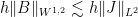
The Laplace equation. We start by introducing the $L^p$ norms informally: we discuss no duality theory and appeal to no measure theory, but only state the Hoelder and Minkowski inequalities, and take completeness as a black box. We similarly define the $C^r$ norms.

We now introduce the Dirichlet energy $I[u] = ||\nabla u||_{L^2}^2$ in several different forms: a quantity that is minimized by a chemical system in equilibrium, a term in the Mumford-Shah energy from image processing, and a linear approximation to the Lagrangian action $||\sqrt{1 + |\nabla u|^2}||_{L^1}$ for minimal graphs. The case of minimal graphs would be particularly fun to teach, as one can bring in bubble wands and try to predict the shapes of soap films, which locally are minimal graphs. (This activity was suggested in a talk of Jenny Harrison.) We then introduce the notions of Lagrangian and Laplacian, and deduce that

Let $u \in C^2$ . Then $I[u]$ is minimal subject to Dirichlet boundary data iff u solves the Laplace equation.

For the sake of later discussion, we also introduce the heat equation as the gradient flow of the Dirichlet energy.

So now we have motivated the Laplace equation. We argue that $I[u]$ is invariant under the rotation group $SO(n)$ , which gives the formula for a Newtonian potential almost immediately. The Dirichlet energy also gives an easy proof of uniqueness for the Laplace equation. We then introduce the notion of convolution, motivated by signal-processing filters. Convolution against Gaussians gives an easy proof that harmonic functions are smooth and convolution against the Newtonian potential solves the Laplace equation. (The reason I want to use Gaussians here is that constructing smooth functions of compact support is an annoying technical argument that not all students may be comfortable with.) We conclude by proving the maximum modulus principle, which implies the fundamental theorem of algebra.

Baby’s first harmonic analysis course. We start with a history lesson: In 1798, Joseph Fourier joins Napoleon Bonaparte on his conquest of Egypt. Twenty-four years later, Fourier releases his controversial treatise on the heat equation, in which he uses some seemingly dubious methods to approximate functions by trigonometric polynomials. Thus it is our job to make right what Dr. Fourier got wrong.

So we introduce the space $C^\infty(T^n)$ of smooth functions on a torus, and argue that we can approximate them using trigonometric polynomials. Here we take the Stone-Weierstrass theorem as a black box. Taking dual spaces, we introduce the Dirac delta function as the unit of convolution and then define periodic distributions. Since this is a course for undergraduates, it is crucial that this step can be carried out without introducing the notion of a Fréchet space, as one just needs to define covectors on $C^\infty(T^n)$ to be those linear maps which satisfy the suitable inequalities. Thus we solve the heat equation subject to smooth initial data and periodic boundary data. We also observe that the Laplace equation has no solutions subject to periodic boundary data except the zero solution.

But, contra to Nietzsche, time is not a flat circle and so we want to solve these equations on euclidean space. So now we introduce the Schwartz space, motivated by our use of $C^\infty(T^n)$ , and the Fourier transform on Schwartz space. We then prove the Fourier inversion formula and introduce the notion of a tempered distribution.

At this point, we hit upon a fundamental theorem:

If a linear PDE is invariant under the group $\mathbb R^n$ , then it is diagonalized by the Fourier transform.

As a corollary, the heat equation is immediately solved. We also give another derivation of the Newtonian potential, using invariance under $\mathbb R^n$ rather than $SO(n)$ this time.

—-

At this point we’re probably a third of the way through the semester, and have touched upon several key themes: the use of the Fourier transform to solve equations, the importance of the symmetry group, and the importance of estimates. Now it is time for the students to pick topics for us to cover for the rest of the semester, based on their interests, since we certainly will not have time to study them all. We pick from:

The wave equation and Einstein’s theory of special relativity. Taking the Maxwell equation as a given, we deduce the curl-of-curl theorem and deduce that the Maxwell equation is actually a system of wave equations. This allows us to carry out Maxwell’s argument that light is an electromagnetic wave.

We now digress to study the wave equation in general. We first show that it arises from the Dirichlet energy if we flip a sign… that may be important later! It is easy to solve the equation subject to initial data and periodic boundary data, since we may use Fourier series; we can also factor the wave equation, which gives the solution on $\mathbb R^n$ subject to initial data. We also prove finite propagation speed and the energy equipartition theorem, the latter a consequence of the Fourier transform. In addition, we show that while the Laplace equation $\Delta u = f$ satisfies the estimate $||u||_{L^2} \leq C||f||_{L^2}$ , no such estimate is available for the wave equation, and I can say something vague here about the symbol being a nondegenerate conic section.

Now we recall the Michelson-Morley experiment, and deduce the causal properties of special relativity from the finite propagation speed of the wave equation. That funny Lagrangian really is the Dirichlet energy, and the wave equation really is the Laplace equation, provided that we get the relationship between space and time correct. As a corollary we deduce time dilation. Finally we introduce the Lorenz group and deduce that the Maxwell equation is invariant under it, thus showing that electricity and magnetism are one and the same.

Traffic flow and ideal fluids. We derive the Burgers equation as a simplified model for traffic flow on highways. We first observe that the Fourier transform doesn’t seem to actually help here, as the equation is quasilinear rather than linear.

We first attack the Burgers equation using the method of characteristics. We develop the theory of characteristics in general as a way to reduce a nonlinear first-order PDE to an ODE, before using them to solve the Burgers equation. We compute the blowup time, which gives a proof that subject to suitable initial data, traffic shockwaves must exist. We then give some numerical simulations to show the effect of traffic shockwaves on a traffic jam.

Having run into the issue of finite blowup time, we now go back to the Burgers equation and show that it is also the one-dimensional case of the Euler equation for an ideal fluid. Adding a viscosity term, we argue that the Burgers equation is actually a sort of nonlinear heat equation. Using the Cole-Hopf transform, we rewrite the Burgers equation as a heat equation and solve using the Fourier transform. We then talk about the vanishing-viscosity limit approximation to the traffic (inviscid) case, and when it is valid.

This lecture series would be somewhat open-ended, as students can come up with their own traffic flow models for the class to analyze, adding, e.g., terms to account for the possibility of an accident to Burgers’ equation.

Finite abelian groups and numerical analysis. Since I think an algebra class will not be a prerequisite, we first summarize the basics of finite abelian groups, and take their classification as a black box. We then discuss the Fourier transform on finite abelian groups, and argue that it converges to the Fourier series on a suitable torus in the large-order limit. Analogously to the theorem on $\mathbb R^n$ -invariant PDE, we argue that circulant matrices are diagonalized by the Fourier transform. We then discuss the fast Fourier transform, and its numerical applications.

More on variational calculus. We develop the theory of variational calculus, and give sufficient conditions on a Lagrangian for its Euler-Lagrange equation to have a solution. This of course requires us to take the dominated convergence theorem and Sobolev trace theorems as black boxes. As applications, we show that many equations have solutions, and give a short proof of Brouwer’s fixed point theorem.

We then digress to define the notion of a Lie group. Since this is an undergraduate course, we just consider Lie groups which are smoothly embedded in $\mathbb R^n$. We then prove Noether’s theorem on the symmetries of Lagrangians, the “fundamental theorem of physics”.

Heisenberg’s uncertainty principle. We first introduce the Schrödinger equation and solve it using separation of variables and the Fourier transform. This reduces all questions of quantum mechanics to questions about the spectrum of the Hamiltonian, so we discuss quantum mechanics for a bit, and in particular how one can use the spectral theorem (taken as a black box) and the Laplacian to study quantum mechanics. This naturally leads to the question of “hearing the shape of a drum”, which is hard, so we do not try to answer it. If I remember correctly, however, one can at least prove Weyl’s law on the distribution of eigenvalues using fairly low-tech methods. We then prove Heisenberg’s uncertainty principle for functions in $L^2$ . We do not, however, dare try to give a physical interpretation of it, other than the music-theoretic interpretation.

Some common beginners’ proof errors

Recently, both through grading proofs and trying to teach some new math majors how to write proofs, I’ve had the opportunity to see a lot of invalid proofs. I want to record here some of the more common errors that invalidate an argument here.

Compilation errors. When grading a huge stack of problem sets, I kind of feel like a compiler. I go through each argument and stop once I run into an error. If I can guess what the author meant to say, I throw a warning (i.e. take off points) but continue reading; otherwise, I crash (i.e. mark the proof wrong).

So by a compilation error, I just mean an error in which the student had an argument which is probably valid in their heads, but when they wrote it down, they mixed up quantifiers, used an undefined term, wrote something syntactically invalid, or similar. I believe that these are the most common errors. Here are some examples of sentences in proofs that I would consider as committing a compilation error:

For a conic section $C$ , $\Delta = b^2 - 4ac$ .

Here the variable $\Delta,a,b,c$ are undefined at the time that they are used, while the variable $C$ is never used after it is bound. From context, I can guess that $\Delta$ is supposed to be the discriminant of $C$ , and $C$ is supposed to be the conic section in the $(x,y)$ -plane cut out by the equation $ax^2 + bxy + cy^2 + dx + ey + f = 0$ where $(a,b,c,d,e,f)$ are constants. So this isn’t too egregious but it is still an error, and in more complicated arguments could potentially be a serious issue.

There’s another thing problematic about this example. We use “For” without a modifier “For every” or “For some”. Does just one conic section satisfy the equation $\Delta = b^2 - 4ac$ , or does every conic section satisfy this equation? Of course, the author meant that every conic section satisfies this equation, and in fact probably meant this equation to be a definition of $\Delta$ . So this compilation error can be fixed by instead writing:

Let $C$ be the conic section in the $(x,y)$ -plane defined by the equation $ax^2 + bxy + cy^2 + dx + ey + f = 0$ . Then let $\Delta = b^2 - 4ac$ be the discriminant of $C$ .

Here’s another compilation error:

Let $V$ be a $3$ -dimensional vector space. For every $x, y \in V$ , define $f(x, y) = xy$ .

Here the author probably means that $f(x, y)$ is the cross-product, or the wedge product, or the polynomial product, or the tensor product, or some other kind of product, of $x,y$ . But we don’t know which product it is! Indeed, $V$ is just some three-dimensional vector space, so it doesn’t come with a product structure. We could fix this by writing, for example:

Let $V = \mathbb R^3$ , and for every $x, y \in V$ , define $f(x, y) = x \times y$ for the cross product of $x,y$ .

We have seen that compilation errors are usually just caused by sloppiness. That doesn’t mean that compilation errors can’t point to a more serious problem with one’s proof — they could, for example, obscure a key step in the argument which is actually fatally flawed. Arguably, this is the case with Shinichi Mochizuki’s infamous incorrect proof of Szpiro’s Conjecture. However, I think that most beginners can avoid compilation errors by making sure that they define every variable before using it, are never ambiguous about if they mean “for every” or “for some”, and otherwise just being very careful in their writing. And beginners should avoid using symbol-soup whenever possible, in favor of the English language. If you ever write something like

Suppose that $f: ~\forall \varepsilon > 0 \exists \delta > 0 \forall(x,y:|x-y| < \delta) (|f(x) - f(y)| < \varepsilon)$ .

I will probably take off points, even though I can, in principle, parse what you’re trying to say. The reason is that you could just as well write

Suppose that $f: A \to \mathbb R$ is a function, and for every $\varepsilon > 0$ we can find a $\delta > 0$ such that for any $x, y \in A$ such that $|x - y| < \delta$ , $|f(x) - f(y)| < \varepsilon$ .

which is much easier to read.

Edge-case errors. An edge-case error is an error in a proof, where the proof manages to cover every case except for a single special case where the proof fails. These errors are also often caused by sloppiness, but are more likely to actually be a serious flaw in an argument than a compilation error. They also tend to be a lot harder to detect than compilation errors. Here’s an example:

Let $f: X \to Y$ be a function. Then there is some $y \in Y$ in the image of $f$ .

Do you see the problem? Don’t read ahead until you try to find it for a few minutes.

Okay, first of all, if you read ahead without trying to find the problem, shame on you; second of all, if you’ve written something like this, don’t feel shame, because it’s a common mistake. The issue, of course, is that $X$ is allowed to be the empty set, in which case $f$ is the infamous empty function into $Y$ .

Most of the time the empty function isn’t too big of an issue, but it can come up sometimes. For example, the fact that the empty function exists means that arguably $0^0 = 1$ , which is problematic because it means that the function $x \mapsto 0^x$ is not continuous (since if $x > 0$ then $0^x = 0$ ).

Here’s an example from topology:

Let $X$ be a connected space and let $x_1,x_2 \in X$ . Then let $\gamma$ be a path from $x_1$ to $x_2$ .

In practice, most spaces we care about are quite nice — manifolds, varieties, CW-complexes, whatever. In such spaces, if they are connected we can find a path between any two points. However, this is not true in general, and the famous counterexample is the topologist’s sine curve. The point is that it’s very important to make sure you get your assumptions right — if you wrote this in a proof there’s a good chance it would cause the rest of the argument to fail, unless you had an additional assumption that the space $X$ did in fact have the property that connected implied path-connected.

In general, a good strategy to avoid errors like the above error is to beware of the standard counterexamples of whatever area of math you are currently working in, and make sure none of them can sneak past your argument! One way to think about this is to imagine that you are Alice, and Bob is handing you the best counterexamples he can find for your argument. You can only beat Bob if you can demonstrate that none of his counterexamples actually work.

Let me also give an example from my own work.

Let $X$ be a bounded subset of $\mathbb R$ . Then the supremum of $X$ exists and is an element of $\mathbb R$ .

It sure looks like this statement is true, since $\mathbb R$ is a complete order. But in fact, $X$ could be the empty set, in which case every real number is an upper bound on $X$ and so $\mathrm{sup } X = -\infty$ . In most cases, the reaction would be “So what? It’s just an edge case error.” But actually, in my case, I later discovered that the thing I was trying to prove was only interesting in the case that $X$ was the empty set, in which case this step of the argument immediately fails. A month later, I’m still not sure what to do to get around this issue, though I have some ideas.

Fatal errors. These are errors which immediately cause the entire argument to fail. If they can be patched, so much the better, but unlike the other two types of errors that can usually be worked around, a fatal error often cannot be repaired.

The most common fatal error I see in beginners’ proofs is the circular argument, as in the below example:

We claim that every vector space is finite-dimensional. In fact, if $\{v_1, \dots, v_n\}$ is a basis of the vector space $V$ , then $\mathrm{dim }V = n < \infty$ , which proves our claim.

If you read a standard textbook on linear algebra, they will certainly assume that given a vector space $V$ , you can find a basis $\{v_1, \dots, v_n\}$ of $V$ . But in fact, such a finite basis only exists if, a priori, $V$ is finite-dimensional! So all the student here has managed to prove is that if $V$ is a finite-dimensional vector space, then $V$ is a finite-dimensional vector space… not very interesting.

(This is not to say that there are almost-circular arguments which do prove something nontrivial. Induction is a form of this, as is the closely related “proof by a priori estimate” technique used in differential equations. But if one looks closely at these arguments they will see that they are not, in fact, circular.)

The other kind of fatal error is similar: there’s some sneaky assumption used in the proof, which isn’t really an edge case assumption. I have blogged about an insidious such assumption, namely the continuum hypothesis. In general, these assumptions often are related to edge-case issues, but may even happen in the generic case, as you mentally make an assumption that you forget to keep track of. Here is another example, also from measure theory:

Let $X$ be a Banach space and let $F: [0, 1] \to X$ be a bounded measurable function. Then we can find a sequence $(F_n)$ of simple measurable functions such that $F_n \to F$ almost everywhere pointwise and $(F_n)$ is Cauchy in mean, so we define $\int_0^1 F(x) ~dx = \lim_{n \to \infty} \int_0^1 F_n(x) ~dx$ .

This definition looks like the standard definition of an integral in any measure theory course. However, without a stronger assumption on $X$ , it’s just nonsense. For one thing, we haven’t shown that the definition of $\int_0^1 F(x) ~dx$ doesn’t depend on the choice of $(F_n)$ . That can be fixed. What cannot be fixed is that $(F_n)$ might not exist at all! This happens if $X$ is not separable, in which case the definition of the integral is nonsense.

This sort of fatal error is particularly tricky to deal with when one is first learning a more general version of a familiar theory. Most undergraduates are familiar with linear algebra, and the fact that every finite-dimensional vector space has a basis. In particular, every element of a vector space can be written uniquely in terms of a given basis. So when one first learns about finite abelian groups, they might be tempted to write:

Let $G$ be a finite abelian group, and let $g_1, \dots, g_n$ be a minimal set of generators of $G$ . Then for every $x \in G$ there are unique $x_1, \dots, x_n \in \mathbb Z$ such that $x = x_1g_1 + \cdots + x_n g_n$ .

In fact, the counterexample here is $G = \mathbb Z/2$ , $n = 1$ , $g_1 = 1$ , and $x = 0$ , because we can write $0 = 0g_1 = 2g_1 = 4g_1 = \cdots$ . So, when generalizing a theory, one does need to be really careful that they haven’t “imported” a false theorem to higher generality! (There’s no shame in making this mistake, though; I think that many mathematicians tried to prove Fermat’s Last Theorem but committed this error by assuming that unique factorization would hold in certain rings — after all, unique factorization holds in everyone’s favorite ring $\mathbb Z$ — that it fails in.)

What the hell is a Christoffel symbol?

I have to admit that I’ve gone a long time without really understanding the physical interpretation of the Christoffel symbols of a connection. In fact, there is an interpretation that, in the special case of the Christoffel symbols for the Levi-Civita connection in polar coordinates on Euclidean space, could be understood by me at age 16, after I took an intro physics class (though I definitely wouldn’t understand the relativistic or Yang-Millsy stuff). Here I want to record it. As usual, I’m pretty sure that everything here is very well-known, but I want to write it all down for my own intuition.

Let D be the covariant derivative of a connection on a vector bundle E. Given a coordinate frame e, one defines the Christoffel symbols by $D_j e_k = {\Gamma^i}_{jk} e_i$ . Here and always we use Einstein’s convention.

The Levi-Civita connection. Suppose E is the tangent bundle of spacetime and D is the Levi-Civita connection of the metric. Then for any free-falling particle with velocity v and acceleration a, one has the relativistic form of Newton’s first law of motion $a^k + {\Gamma^k}_{ij} v^iv^j = 0$ , which to mathematicians is more popularly known as the geodesic equation. It says that the “acceleration” in the coordinate frame e is entirely due to the fact that e itself is an accelerated frame.

Viewing $\Gamma^k$ as a bilinear form, we can rewrite Newton’s first law as $a^k = -\Gamma^k(v, v)$ , which now resembles Newton’s second law with unit mass. Indeed, the acceleration of the particle is given exactly by a quantity $-\Gamma^k(v, v) e_k$ which can be reasonably interpreted as a “force”. For example, one could consider the case that the spatial origin is a particle P which is orbiting around a point. If one believes that P really is “inertial”, then they will measure a fictitious force — the centrifugal force — acting on all objects. In general relativity, moreover, I think that the notion of “inertial” is ill-defined. In this case, if v is timelike then $\Gamma^k(v, v)$ is the acceleration due to gravity. In particular these fictitious forces all scale linearly with mass, because the geodesic equation does not have a mass factor and so we need to cancel out the factor of mass in the law $F = ma$ .

It will be convenient to go to another level of abstraction and view $\Gamma: T_pM \otimes T_pM \to T_pM$ as a quadratic form valued in the tangent space. In other words it is tempting to think of $\Gamma$ as a section of $T^*M \otimes T^*M \otimes TM$ . This of course presupposes that M has a trivial tangent bundle, since the Christoffel symbols are only defined locally. Putting our doubts aside, this is equivalent to thinking of $\Gamma$ as a section of $T^*M \otimes \text{End } TM$ .

Connections on G-bundles. Let me remind you that if G is a Lie group, then a G-bundle is a bundle of representations of G. Thus we can view quotients of G and its Lie algebra $\mathfrak g$ as both subsets of End E, whenever E is a G-bundle. By a gauge transformation of a G-bundle E one means a section of End E which is in fact a section of G. Thus gauge transformations act on E (and so also on End E, etc.)

If E is a G-bundle, by a covariant derivative on E I mean a covariant derivative whose Christoffel symbols $\Gamma$ are not just sections of $T^*M \otimes \text{End } E$ but in fact are sections of $T^*M \otimes \mathfrak g$ . (Briefly, the Christoffel symbols are $\mathfrak g$ -valued 1-forms.) In this case, if we have two covariant derivatives D, D’ which lie in the same orbit of the gauge transformations, we call D, D’ gauge-equivalent. We tend to think of covariant derivatives of G-bundles (modulo gauge-equivalence) as describing physical theories.

For example, consider the trivial U(1)-bundle E. This is the trivial line bundle equipped with the canonical action of U(1) on the complex numbers. A covariant derivative D on E is defined by locally giving Christoffel symbols which are $\mathfrak u(1)$ -valued 1-forms — in other words, imaginary 1-forms. A gauge transformation, then, is defined by adding an imaginary exact 1-form to the Christoffel symbols. We interpret the Christoffel symbols A as (i times) potentials for the electromagnetic field. In fact, one can take the exterior derivative of A and obtain a closed 2-form $F = dA$ , which one can view as the Faraday tensor. The fact that one can add an exact 1-form to A is exactly the gauge invariance of the Maxwell equation $*d*dA = j$ where j is the current 1-form.

So what is D in the case of electromagnetism? It acts on sections as $D_i = \partial_i + A_i$ . So for a function u (i.e. a section of the trivial bundle E) on M, $(D_i - \partial_i)u$ weights u according to the strength of the electromagnetic potential. This is mainly interesting when u is a constant function, in which case $Du = uA$ is the potential rescaled by u.

I think that the takeaway here is: the Christoffel symbols are a fictitious and local V-valued 1-form, where V is some vector bundle ( $V = \mathfrak g$ or $V = TM \otimes T^*M$ above). In any particular case they should have a nice physical interpretation but I don’t think one can interpret the Maxwell-Yang-Mills case and the Levi-Civita case as one and the same.